Network Analysis

-
Nodes Labels:
-
Assault, Burglary, Death, Fraud, Robbery, Sexual, Theft, Drug
-
-
Number of Nodes: 8
-
Number of Edges: 55
-
Density: 0.982143
-
Degree of Each Node:
-
13, 14, 14, 14, 14, 14, 14, 13
-
-
KNN:
-
76.935707, 4.612677, 152.915874, 20.746856, 14.095713, 157.406189, 3.840974, 19.166044
-
-
Eigenvector Centralities:
-
0.036921, 1.0, 0.002108, 0.115819, 0.168534, 0.001483, 0.824035, 0.116584
-
-
Betweenness:
-
25.0, 0.0, 6.0, 8.0, 0.0, 25.0, 0.0, 0.0
-
-
The Local Transitivity (Clustering Coefficient):
-
0.733503, 1.050825, 0.636321, 0.817849, 0.873051, 0.995601, 0.971484, 0.989918
-
The density is the the fraction of actual connections (edges) divided by all possible connections (edges) in the network (graph). Since, the density for this network is really, it means that almost all different types of crime have been paired up and be the two most frequent crime type in a specific day. The degree is the number of neighbors an individual nodes has. In this case, only Assault and Drug has degree of 13, other crimes all have degree of 14, which means the co-occurrence of Assault and Drug compared to other crime types is lower.
The edge weights are the strength of the relationship between two nodes, which are the numbers one the lines in the network graph. The thicker the line, the heavier the weights are. Thus, from the above graph, crime like Burglary and Theft are linked with heavy lines, which indicate that there exist a strong relationship between the two crimes. It may also infer that the two crime type are similar in some way.
The KNN will take weights into consideration and calculate the average degree of the neighbors for each vertex. And Death and Sexual crime have the highest KNN, which means that the two crimes are less weighted and do not occur as often as other crimes. The eigenvector centralities calculate the centralities of the vertices in a graph. From the results above, Burglary and Theft, which has the highest centralities, could have a considerable influence within the network by virtue of their control over information passing between others.
The eigenvector centralities calculate the centralities of the vertices in a graph. From the results above, Burglary and Theft, which has the highest centralities, could have a considerable influence within the network by virtue of their control over information passing between others.
The local transitivity or clustering coefficient calculates the probability that two neighbors of a vertex are connected; in this case, this probability is calculated separately for each vertex. From the output above, it is more likely that Burglary, Robbery, Theft and Drug are more likely to be clustered together.
Spatial temporal analysis with Monte Carlo Approach
Theft Crime Spatial Temporal Pattern in LA
Theft Crime Spatial-Temporal Pattern in LA

From this map, the dark green shows that the occurrence of Theft crime in Weekend is significantly higher than the corresponding in the rest of week.The red shows that the occurrence of Theft crime in Weekend is significantly higher than the corresponding in the rest of week. the light green shows that there is no significant difference between weekend and the rest of days in the week. In this way, from this graph , compared to the graph 9, even though the distribution of theft type in different days shows that the theft crime rates in the weekday is generally higher than weekday, the results is different when considering spatial pattern. For example, statistically, in the spatial pattern around Santa Monica area which is the recreation parking area, the theft crime rate is significantly higher on weekend than the crime on weekday.
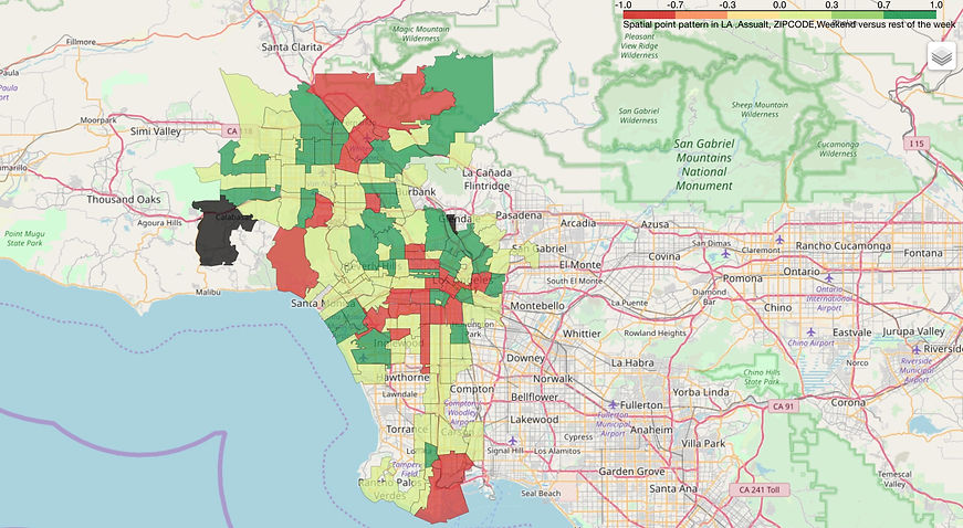
Assault Crime Spatial-Temporal Pattern in LA

From this map, the dark green shows that the occurrence of Assault crime in Weekend is significantly higher than the corresponding in the rest of week.The red shows that the occurrence of Assault crime in Weekend is significantly higher than the corresponding in the rest of week. the light green shows that there is no significant difference between weekend and the rest of days in the week. In this way, from this graph , compared to the graph 9, even though the distribution of Assault type in different days shows that the Assault crime rates in the weekday is generally lower than weekday, the results is different when considering spatial pattern. For example, statistically, even though the numbers of dark green units are more than numbers of red green units, compared to the graph 9, there are still some large area with the opposite results that is red area, it means some specific area with the lower Assault crime on weekend.